
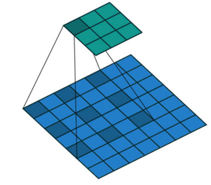
Convolution
It’s a technique that allows us to detect patterns in a multi-dimensional data without flattening it into a 1D vector.
A kernel (or filter) is a small matrix of numbers (learnable weights) that detects certain patterns. It slides over the data, one small patch at a time.
The convolution is the process of taking the dot product between the kernel and each region of the input. The result is a smaller grid called a feature map or activation map, containing the responses of the kernel at each location.
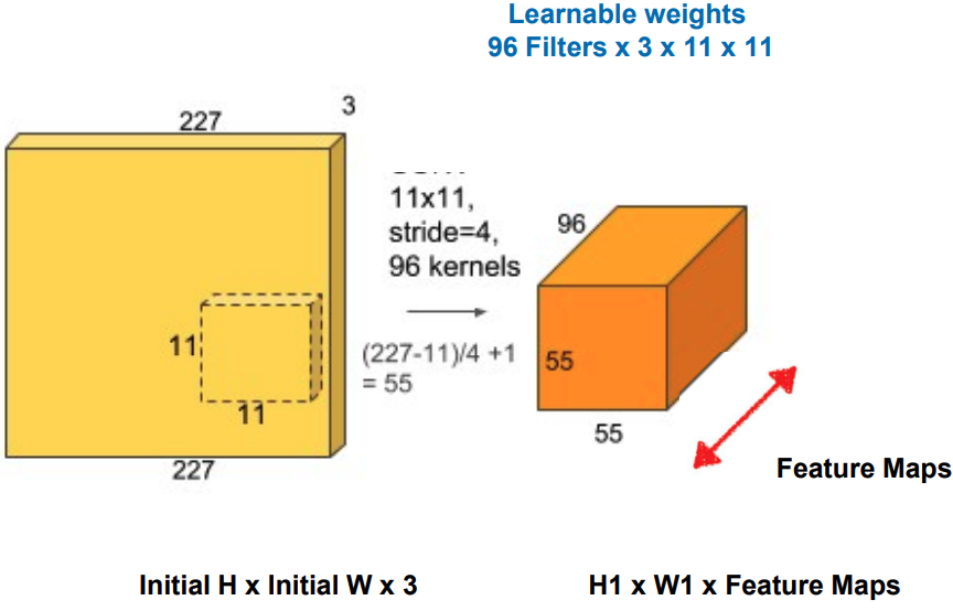
A convolutional layer contains many filters/kernels, as each kernel will need to extract different patterns/features. A filter is a small set of weights (e.g. 11×11×3) that detects one pattern. Each of these filters outputs 1 channel.
Padding
We usually pad an image by adding a border of pixels (zero or duplicates). This keeps the dimensions the same and avoids losing border information.
Strides
How many pixels we move the kernel each step
Convolution Layer
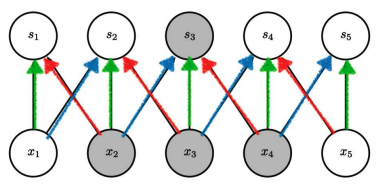 A CNN doesn’t have a lot of weights. In this example, only 3 learnable weights because every output neuron applies the same kernel.
The same feature (a vertical edge) can appear anywhere, and the filter will detect it. This creates translation equivariance (if an object moves, the feature map moves too)
This parameter efficiency enables deeper networks,
A CNN doesn’t have a lot of weights. In this example, only 3 learnable weights because every output neuron applies the same kernel.
The same feature (a vertical edge) can appear anywhere, and the filter will detect it. This creates translation equivariance (if an object moves, the feature map moves too)
This parameter efficiency enables deeper networks,
Receptive Fields
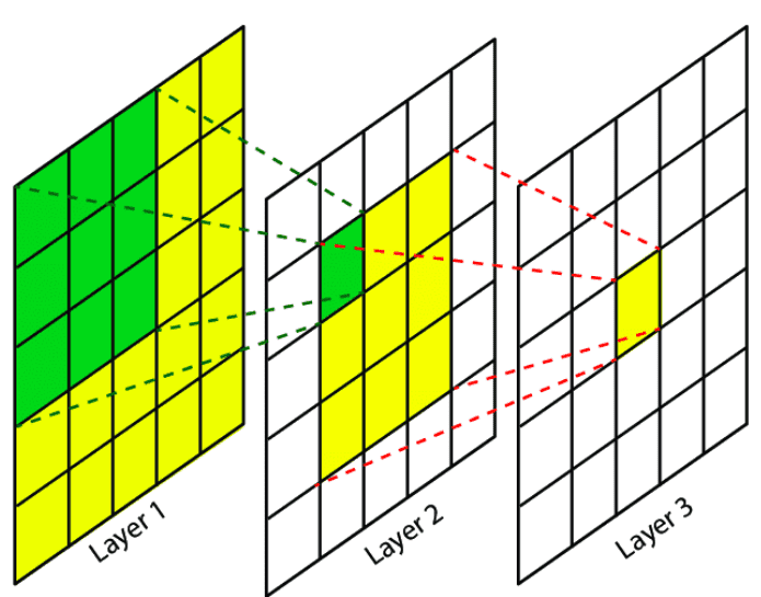 Initially, a neuron might only see the size of a single kernel, but in deeper layers, each neuron ends up seeing a larger portion of the original image.
This means that deeper layers detect higher-level concepts (eyes → face → head → person) because their receptive fields grow.
Initially, a neuron might only see the size of a single kernel, but in deeper layers, each neuron ends up seeing a larger portion of the original image.
This means that deeper layers detect higher-level concepts (eyes → face → head → person) because their receptive fields grow.
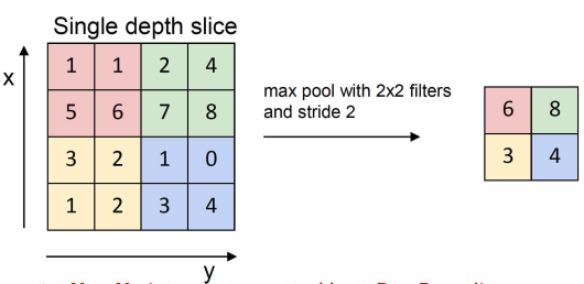
Pooling
Pooling lets you reduce the spatial size (HxW) of feature maps while keeping channels the same. It’s basically down-sampling.
You can pool a 2x2 into 1 value, choosing the max or the avg of the 4.
 They help with:
- translation invariance
- network becomes less sensitive to small shifts in the image
- dimensionality reduction
- fewer parameters in later layers → less overfitting
- increasing RF (receptive field)
- pooling expands each neuron’s influence backwards thru image
AlexNet
The first deep CNN.
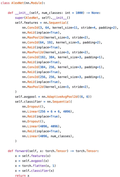 The first convolutional layer (CONV1) has a kernel size of 11 to aggressively reduce the spatial resolution.
At the end we have a few fully-connected layers (this is where the huge parameter count comes from) for imagenet classification.
The first convolutional layer (CONV1) has a kernel size of 11 to aggressively reduce the spatial resolution.
At the end we have a few fully-connected layers (this is where the huge parameter count comes from) for imagenet classification.
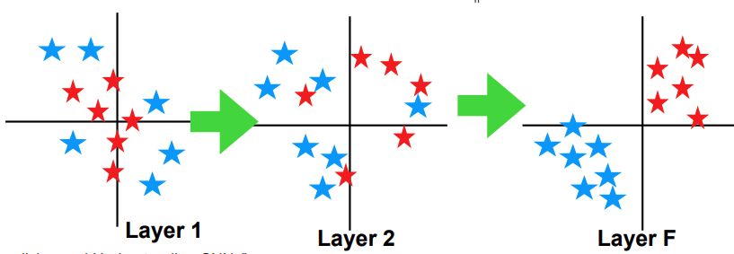
Higher-level features are more semantically meaningful and we can actually separate them with a linear classifier.
Residual Learning
Deeper neural networks suffer from vanishing gradients and a degradation problem where the training error actually increases as we add layers.
One possible solution might be residual learning, where we actually skip certain layers.
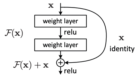 , if a residual block learns , it then adds the original input , so that the block learns the change to the input, not a whole transormation.
If we unroll all the possible skip connections, we get many paths, each path resembling a smaller, simpler network. This improves robustness, generalization and optimization.
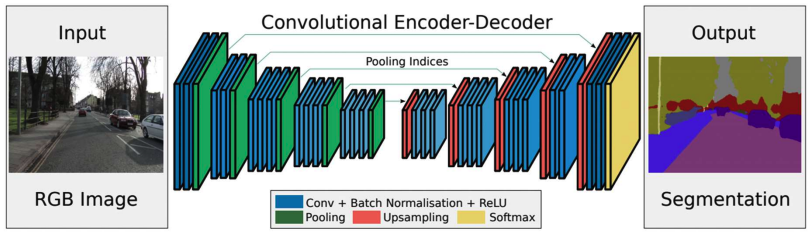
Semantic Segmentation and Fully Convolutional Networks (FCNs)
In semantic segmentation, instead of assigning one label per image (classification) we assign one label per pixel.
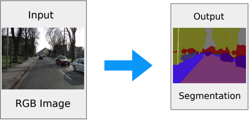 A classical CNNs that ends with fully connected layers destroy spatial resolution and are unusable for segmentation.
A FCN replaces these fully connected layers with 1x1 convolutions, that keep spatial structure and perform per-pixel classification.
Then, we’ll upsample to recover full resolution.
A classical CNNs that ends with fully connected layers destroy spatial resolution and are unusable for segmentation.
A FCN replaces these fully connected layers with 1x1 convolutions, that keep spatial structure and perform per-pixel classification.
Then, we’ll upsample to recover full resolution.
dilations
A dilation rate determines the spacing between kernel elements. Normal convolutions have a dilation of 0. Here’s an example of a dilation of 1:
 It increases receptive field without reducing resolution, pooling or increasing parameters.
This is crucial in segmentation because you want large context, and full-resolution feature maps.
It increases receptive field without reducing resolution, pooling or increasing parameters.
This is crucial in segmentation because you want large context, and full-resolution feature maps.
not only 2d conv nets
1d conv nets: audio, time series, text (before transformers) 3d conv nets: medical imaging, video understanding, shape classification