
some of these notes from: jordan has no life
Hash Indices
Hashmap
We know a hash function spits out a number (hash) in range, given an input. If two elements are hashed in the same place, instead of a key you can put a linked list for each element in your table. Otherwise you could put it in the next free element, with a load factor it’s still amortized constant time.
Why don’t databases use hashmaps if they’re constant time for read and writes?
- They’re bad on disk. Because in a hashmap the data is distributed evenly and not close to each other. So the performance is poor on disks because the disk arm jumps around.
- Can’t put hashmaps on memory, RAM is expensive. Keys won’t fit on a ram. Also ram isnt durable lol.
- We could use ram for indexes by putting all operation on a WAL (Write Ahead Log), so if the DB dies we can re-populate our indexes.
- WAL provides durability in other types of indexes too.
- We can’t do range queries either. If we want all rows with even ID, we’d have to loop over every even number so it’s still O(n).
TLDR hash index is good if we have a relatively small amount of keys to keep in memory, we want O(1) reads/writes, and we dont need range queries.
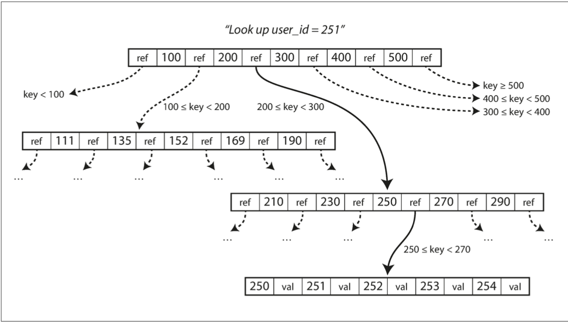
B-Trees
Basically a tree traversal. Each node has a range of values and a reference to each range. For reads, just traverse the tree, for writes, find an empty leaf to put your value in. If the leaf is full, you have to traverse up the tree and split the ranges until it fits.
The branching factor is the number of references we keep per page. Usually it’s several hundred.
Overall, good in terms of read, just a couple of traversal on disk Advantages over hash indices:
- not all of the keys have to be fit in memory, can have larger dataset
- we can do range queries! Disadvantages:
- slower, large portion of keys have to be on disk. writes not super fast
- write to WAL, then go to bottom of tree, then may have to traverse all the way back up the tree switching references on disks.
- updating might be slow as if page is full you’d have to write 2 new pages and then update the parent pages references too.
SSTables and LSM-Trees
An LSM tree is another type of DB index, similar to a AVL / B-tree / Red-black tree, any balanced binary search tree that is going to be put in memory.
Again, O(logn) for reads and write, but unfortunately it’s in memory:
- no durability
- We’ll use a WAL, at the cost of slower writes coz gotta write to disk too
- less space
- Let’s say our LSM tree gets too full, we’ll reset it and put its contents into a sorted list immutable SSTable (to get sorted list just do in-order traversal on list)
- So now when reading we gotta incorporate our SSTables (Sorted String Tables). We first read from LSM tree, if it’s not there, we look for the key in our SSTables (multiple as one can get full).
- As we said SSTables are immutable therefore to delete a key we just add it again to the most recent SSTable with a “tombstone” value.
- The nice thing about SSTables is that they’re sorted so we can just binary search to read. So, all in all reads are O(logn). If the db crashes, we’ll lose our lsm tree! Not necessarily, we’ll keep a WAL and then reset it whenever we dump our lsm tree to a sstable.
Optimizations
Instead of checking LSM tree first, then if key isnt there check SSTable etc, we can add 2 optimizations:
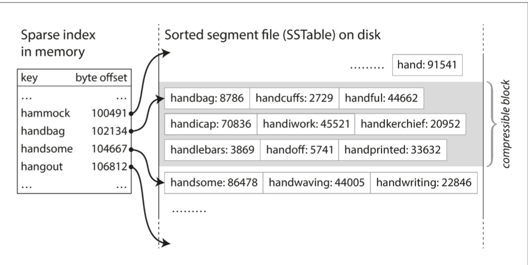
- SPARSE INDEX: We can take certain keys and write their location on disk. We can say: “A” starts at 0x000, J starts at 0x11f, S at 0x2ab, Q at 0x3c6. Then when we read from this SSTable we can just see in what range our filter falls into and start our binary search from there already.
- BLOOM FILTER: This is needed because checking for a non-existant key is a slow process. We then implement a filter that tells you if a key is 100% not in the set. It may have false positives. Is “X” in sstable? No! definitely correct. Yes! may be wrong. Works by hashing keys, sampling bits from the hash and setting them in a bitfield. On a lookup operation, we check if the hashed key was entered before.
Compaction
If there’s no hard deletion, sometimes we can do compaction. This means sometimes we compact multiple SSTable by only keeping the most recent values. We do this by basically comparing 2 SSTables together by using a two-pointer algorithm. Merge 2 sorted lists. This is good for reducing disk usage that we use.
Conclusion
Hash Index
- PRO: constant read and write
- CON: Keys need to fit in memory
- CON: No range queries allowed
B-Tree
- PRO: fast range queries.
- everything is colocated to similar keys on disk.
- alex and adam are close together on disk.
- PRO: Number of keys not limited in memory
- CON: writes a slightly slower coz you may need to iterate over tree multiple times.
LSM Tree
- PRO: number of keys not limited by memory
- MID: faster writes than B-tree (they go to memory, although WAL too), slower than hash index
- MID: supports range queries but slower than B-trees on reads, because you need to check all SSTables
- CON: Extra CPU usage for compaction.
Wrap up Indices give you faster reads on a specific key, although slower writes for any possible writes. Of course, we’ve been thinking of indices as an abstraction kinda. In the sense that whenever we have an index table for example, all those indices store the memory address of the related data, not the actual data. This way we don’t need to duplicate the data for each index we have ofc.
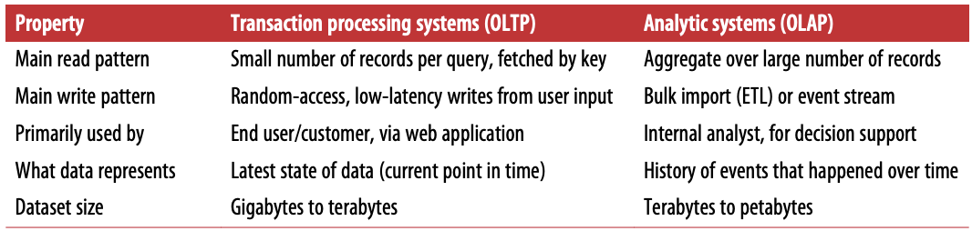
OLTP vs OLAP
A transaction doesn’t necessarily have to have ACID properties. Transaction processing just means allowing clients to make low-latency reads and writes, as opposed to batch processing jobs.
 SQL databases although born for OLTP necessities, actually work quite well for OLAP. Nevertheless, OLTP systems shouldn’t be used for analytics, and a need for a separate database (called a data warehouse) came up.
You can’t run OLAP queries on an OLTP database because you’re gonna slow it down with expensive queries, and it needs to be fast because its main purpose is allowing low latency reads/writes.
SQL databases although born for OLTP necessities, actually work quite well for OLAP. Nevertheless, OLTP systems shouldn’t be used for analytics, and a need for a separate database (called a data warehouse) came up.
You can’t run OLAP queries on an OLTP database because you’re gonna slow it down with expensive queries, and it needs to be fast because its main purpose is allowing low latency reads/writes.
Extract-Transform-Load (ETL)
This is the process of getting data into the warehouse.
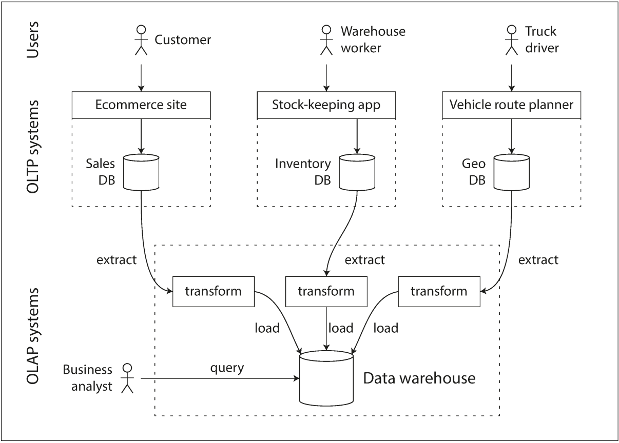 Data warehouses and OLTP databases share the same SQL query interface, but the internals of the systems look different.
Stars and Snowflakes
Data warehouses have pretty simple schemas. Usually a fact table that represents events that occurred at a particular time (this allows maximum flexibility for analysis). STAR SCHEMA: While fact tables represents an event, they have foreign key references to dimension tables that represent the who, what, where, when, how and why of an event. SNOWFLAKE SCHEMA: Dimensions have FK references to other sub-dimension tables.
Column Oriented Storage
These tables can be very wide (hundreds of columns), but every analytics query may only need to access 4 or 5 of them at once. If we store each column in a separate file, a query only needs to read and parse those columns that are used in that query, which can save a lot of work (in row-oriented storage, would need to load all the columns into memory, parse them, and filter out the ones that don’t meet the required conditions). We can further optimize the memory needs for a column oriented storage by compressing the column data into bitmap. Since the number of unique values might be in the hundreds of thousands (instead of billions of rows), we can have a bitmap for each unique value, and then 1 bit per row indicating whether that row has that value or not. If we have sparse bitmaps (lots of zeroes) we can further compress them with run-length encoding.
With this, the CPU can compute bitwise AND and OR on these bitmaps, fitting this data in an L1 cache. This technique is called vectorized processing.
We can also sort rows and use run-length encoding to compress columns that have consequent duplicate values. We just need to remember to sort the rows as a single unit, as we can’t sort a specific column only, as then we’ll lose what row that data belongs to.
A clever way to sort columns is actually storing column data sorted in different ways on different machines. So you can use the data that your query needs the most.
Column oriented storage makes reads very fast but writes complicated due to compression and sorting. You’d need to rewrite the entire column to keep them consisted. We can use the notion from LSM-trees, all writes going to an in-memory store (doesnt matter if row-oriented or column-oriented) and then merge them with column files on disk in bulk.
Data warehouses also cache aggregate functions like COUNT, SUM, AVG, MIN, MAX in materialized views.